The success of Skype has inspired a generation of
peer-to-peer-based solutions for satisfactory real-time
multimedia services over the Internet. However, fundamental
questions, such as whether VoIP services like Skype are good
enough in terms of user satisfaction, have not been formally
addressed. One of the major challenges lies in the lack of
an easily accessible and objective index to quantify the
degree of user satisfaction.
In this work, we propose a model, geared to Skype, but
generalizable to other VoIP services, to quantify VoIP user
satisfaction based on a rigorous analysis of the call duration
from actual Skype traces. The User Satisfaction Index (USI)
derived from the model is unique in that 1) it is composed by
objective source- and network-level metrics, such as the bit
rate, bit rate jitter, and round-trip time, 2) unlike speech
quality measures based on voice signals, such as the PESQ model
standardized by ITU-T, the metrics are easily accessible and
computable for real-time adaptation, and 3) the model development
only requires network measurements, i.e., no user surveys or
voice signals are necessary. Our model is validated by an
independent set of metrics that quantifies the degree of user
interaction from the actual traces.
Human Perception, Internet Measurement, Survival
Analysis, Quality of Service, VoIP, Wavelet Denoising
1 Introduction
There are over 200 million Skype downloads and approximately
85 million users worldwide. The user base is growing at more
than 100,000 a day, and there are 3.5 to 4 million active
users at any one
time23.
The phenomenal growth of Skype has not only inspired a generation
of application-level solutions for satisfactory real-time
multimedia services over the Internet, but also stunned the
market observers worldwide with the recent US$ 4.1 billion
deal with
eBay4.
Network engineers and market observers study Skype for different
reasons. The former seek ways to enhance user satisfaction, while
the latter collect information to refine their predictions of the
growth of the user base. They both, however, need the answer to a
fundamental question: Is Skype providing a good enough
voice phone service to the users, or is there still room
for improvement?
To date, there has not been a formal study that quantifies the level
of user satisfaction with the Skype voice phone service. The
difficulties lie in 1) the peer-to-peer nature of Skype, which
makes it difficult to capture a substantial amount of traffic for analysis; and 2)
existing approaches to studying user satisfaction rely on speech-signal-level information that is not available to parties other
than the call participants. Furthermore, studies that evaluate the
perceptual quality of audio are mostly
signal-distortion-based [11,9,10]. This
approach has two drawbacks: 1) it usually requires access to signals from both ends,
the original and the degraded signals, which is not practical in
VoIP applications; 2) it cannot take account of factors other
than speech signal degradation, e.g., variable listening levels,
sidetone/talk echo, and conversational delay.
We propose an objective, perceptual index for measuring Skype user
satisfaction. The model, called the User Satisfaction Index (USI),
is based on a rigorous analysis of the call duration and source- and
network-level QoS metrics. The specific model presented in this
paper is geared to Skype, but the methodology is generalizable to
other VoIP and interactive real-time multimedia services. Our model
is unique in that the parameters used to construct the index
are easy to access. The required information can be obtained by
passive measurement and ping-like probing. The parameters are also
easy to compute, as only first- and second-moment statistics
of the packet counting process are needed. There is no need to
consider voice signals. Therefore, user satisfaction can be assessed
online. This will enable any QoS-sensitive application to adapt in
real time its source rate, data path, or relay node for optimal
user satisfaction.
To validate the index, we compare the proposed USI with an
independent set of metrics that quantify the degree of voice
interactivity from actual Skype sessions. The basic assumption is
that the more smoothly users interact, the more satisfied they
will be. The level of user interaction is defined by the
responsiveness, response delay, and talk burst length. Speech
activity is estimated by a wavelet-based algorithm [6]
from packet size processes. The strong correlation observed between
the interactivity of user conversations and USI supports the
representativeness of the USI.
By deriving the objective, perceptual index, we are able to quantify
the relative impact of the bit rate, the compound of delay
jitter and packet loss, and network latency on Skype call duration.
The importance of these three factors is approximately
46%:53%:1% respectively. The delay jitter and loss rate are
known to be critical to the perception of real-time applications. To
our surprise, network latency has relatively little effect, but the
source rate is almost as critical as the compound of the delay
jitter and packet loss. We believe these discoveries indicate that
adaptations for a stable, higher bandwidth channel are likely the
most effective way to increase user satisfaction in Skype. The
selection of relay nodes based on network delay optimization, a
technique often used to find a quality detour by peer-to-peer
overlay multimedia applications, is less likely to make a
significant difference for Skype in terms of user satisfaction.
Our contribution is three-fold: 1) We devise an objective and
perceptual user satisfaction index in which the parameters are
all easily measurable and computable online; 2) we validate the
index with an independent set of metrics for voice interactivity
derived from user conversation patterns; and 3) we quantify the
influence of the bit rate, jitter and loss, and delay on call
duration, which provides hints about the priority of the metrics
to tune for optimal user satisfaction with Skype.
The remainder of this paper is organized as follows.
Section 2 describes related works. We discuss the
measurement methodology and summarize our traces in
Section 3. In Section 4, we derive the USI
by analyzing Skype VoIP sessions, especially the relationship
between call duration and source-/network-level conditions. In
Section 5, we validate the USI with an independent set
metrics based on speech interactivity. Finally,
Section 6 draws our conclusion.
2 Related Work
Objective methods for assessing speech quality can be classified
into two types: referenced and unreferenced. Referenced
methods [11,9] measure distortion between
original and degraded speech signals and map the distortion
values to mean opinion scores (MOS). However, there are two
problems with such model: 1) both the original and the degraded
signals must be available, and 2) it is difficult to synchronize
the two signals. Unreferenced models [10], on the
other hand, do not have the above problems, as only the degraded
signal is required. The unreferenced models, however, do not
capture human perception as well as the referenced models.
The USI model and the measures of speech quality although aim
similarly at providing objective metrics to quantify user
perception, however, they have a number of substantial differences:
1) the USI model is based on call duration, rather than speech
quality; therefore, factors other than speech quality, such as
listening volume and conversational delay [11], can also be
captured by USI; and 2) rather than relying on subjective surveys,
the USI model is based on passive measurement, so it can capture
subconscious reactions that listeners are even unaware of.
Table 1 summarizes the major differences.
Table 1: Comparison of the proposed USI and the objective
measures of speech quality
USI
speech quality measures
to quantify
user satisfaction
speech quality
built upon†
call duration
subjective MOS
predictors
QoS factors
distortion of signals
† the response variable used in the model development
3 Trace Collection
In this section, we describe the collection of Skype VoIP sessions
and their network parameters. We first present the network setup and
filtering method used in the traffic capture stage. The algorithm
for extracting VoIP sessions from packet traces is then introduced,
followed by the strategy to sample path characteristics.
Finally, we summarize the collected VoIP sessions.
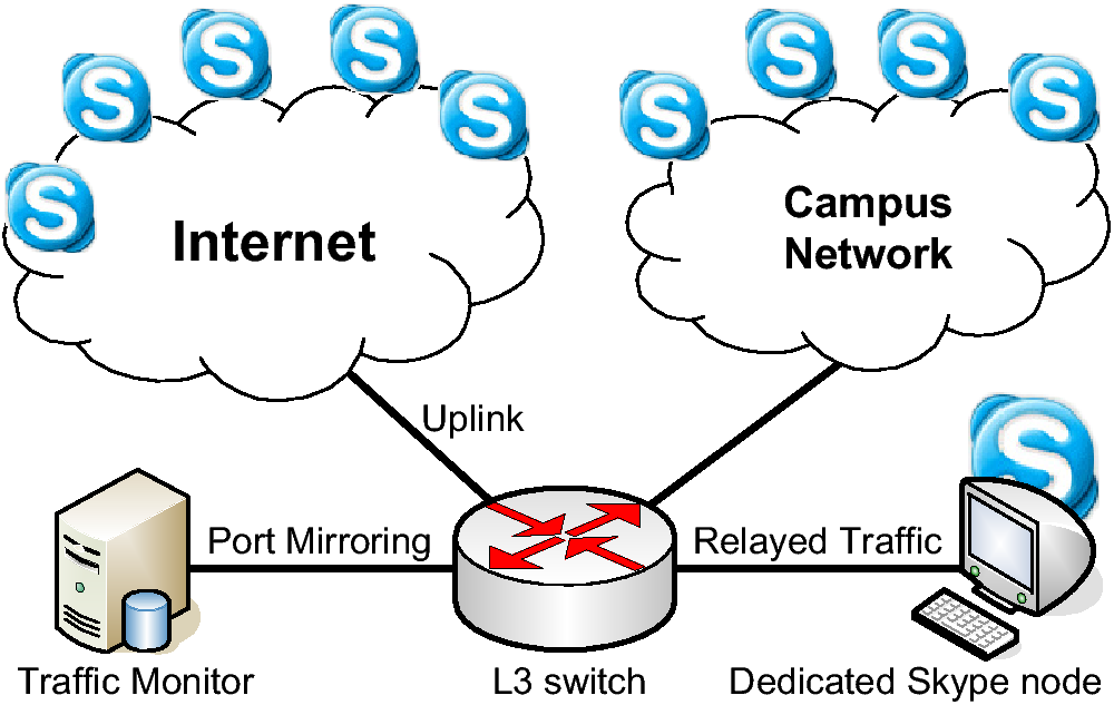
3.1 Network Setup
Because of the peer-to-peer nature of Skype, no one network node can
see traffic between any two Skype hosts in the world. However, it is
still possible to gather Skype traffic related to a particular site.
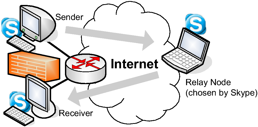
To do so, we set up a packet sniffer that monitors all traffic
entering and leaving a campus network, as shown in
Fig. 1. The sniffer is a FreeBSD 5.2 machine equipped
with dual Intel Xeon 3.2G processors and one gigabyte memory. As
noted in [12], two Skype nodes can communicate via a
relay node if they have difficulties establishing sessions. Also, a
powerful Skype node is likely to be used as the relay node of VoIP
sessions if it has been up for a sufficient length of time.
Therefore we also set up a powerful Linux machine to elicit more
relay traffic during the course of trace collection.
Figure 1: The network setup for VoIP session
collection
3.2 Capturing Skype Traffic
Given the huge amount of monitored traffic and the low proportion of
Skype traffic, we use two-phase filtering to identify Skype VoIP
sessions. In the first stage, we filter and store possible Skype
traffic on the disk. Then in the second stage, we apply an off-line
identification algorithm on the captured packet traces to extract
actual Skype sessions.
To detect possible Skype traffic in real time, we leverage some
known properties of Skype clients [12,1].
First of all, Skype does not use any well-known port number, which
is one of the difficulties in distinguishing Skype traffic from that
of other applications. Instead, it uses a dynamic port number in
most communications, which we call the "Skype port" hereafter.
Skype uses this port to send all outgoing UDP packets and accept
incoming TCP connections and UDP packets. The port is chosen
randomly when the application is installed and can be configured by
users. Secondly, in the login process, Skype submits HTTP requests
to a well-known server, ui.skype.com. If the login is
successful, Skype contacts one or more super nodes listed in
its host cache by sending UDP packets through its Skype port.
Based on the above knowledge, we use a heuristic to detect Skype
hosts and their Skype ports. The heuristic works as follows. For
each HTTP request sent to ui.skype.com, we treat the sender
as a Skype host and guess its Skype port by inspecting the port
numbers of outgoing UDP packets sent within the next 10 seconds.
The port number used most frequently is chosen as the Skype port of
that host. Once a Skype host has been identified, all peers that
have bi-directional communication with the Skype port on that the
host are also classified as Skype hosts. With such a heuristic, we
maintained a table of identified Skype hosts and their respective
Skype ports, and recorded all traffic sent from or to these (host,
port) pairs. The heuristic is not perfect because it also records
non-voice-packets and may collect traffic from other applications by
mistake. Despite the occasional false positives, it does reduce the
number of packets we need to capture to only 1-2% of the
number of observed packets in our environment. As such, it is a
simple filtering method that effectively filters out most unwanted
traffic and reduces the overhead of off-line processing.
3.3 Identification of VoIP Sessions
Having captured packet traces containing possible Skype traffic, we
proceed to extract true VoIP sessions. We define a "flow" as a
succession of packets with the same five-tuple (source and
destination IP address, source and destination port numbers, and
protocol number).
We determine whether a flow is active or not by its moving average
packet rate. A flow is deemed active if its rate is higher than a
threshold 15 pkt/sec, and considered inactive otherwise. The
average packet rate is computed using an exponential weighted moving
average (EWMA) as follows:
Ai+1 = (1 − α)Ai + αIi,
where Ii represents the average packet rate of the i-th
second of the flow and Ai is the average rate. The weight
α is set at 0.15 when the flow is active and 0.75 when
the flow is inactive. The different weights used in different
states allow the start of a flow to be detected more
quickly [12].
An active flow is regarded as a valid VoIP session if all
the following criteria are met:
The flow's duration is longer than 10 seconds.
The average packet rate is within a
reasonable range, (10, 100) pkt/sec.
The average packet size is within (30,300) bytes. Also,
the EWMA of the packet size process (with α = 0.15) must be
within (35,500) bytes all the time.
After VoIP sessions have been identified, each pair of sessions
is checked to see if it can form a relayed session, i.e.,
these two flows are used to convey the same set of VoIP packets
with the relay node in our campus network. We merge a pair of
flows into a relayed session if the following conditions are met:
1) the flows' start and finish time are close to each other with
errors less than 30 seconds; 2) the ratio of their average
packet rates is smaller than 1.5; and 3) their packet arrival
processes are positively correlated with a coefficient higher
than 0.5.
3.4 Measurement of Path Characteristics
As voice packets may experience delay or loss while transmitting
over the network, the path characteristics would undoubtedly affect
speech quality. However, we cannot deduce round-trip times (RTT) and
their jitters simply from packet traces because Skype voice packets
are encrypted and most of them are conveyed by UDP. Therefore,
We send out probe packets to measure paths' round-trip times while
capturing Skype traffic. In order to minimize the possible
disturbance caused by active measurement, probes are sent in batches
of 20 with exponential intervals of mean 1 second. Probe batches
are sent at two-minute intervals for each active flow. While
"ping" tasks are usually achieved by ICMP packets, many routers
nowadays discard such packets to reduce load and prevent attacks.
Fortunately, we find that, certain Skype hosts respond to
traceroute probes sent to their Skype ports. Thus, to
increase the yield rate of RTT samples, traceroute-like
probes, which are based on UDP, are also used in addition to ICMP
probes.
3.5 Trace Summary
The trace collection took place over two months in late 2005. We
obtained 634 VoIP sessions, of which 462 sessions were usable as
they had more than five RTT samples. Of the 462 sessions, 253
were directly-established and 209 were relayed. A summary of the
collected sessions is listed in Table 2. One can see
from the table that median of the relayed session durations is
significantly shorter than that of the direct sessions, as their
95% confidence bands do not overlap.
We believe the discrepancy could be explained by various factors,
such as larger RTTs or lower bit rates. The relationship between
these factors and the session/call duration is investigated in
detail in the next section.
Table 2: Summary of collected VoIP sessions
Category
Calls
Hosts†
Cens.
TCP
Duration‡
Bit Rate (mean/std)
Avg. RTT (mean/std)
Direct
253
240
1
7.1%
(6.43,10.42) min
32.21 Kbps / 15.67 Kbps
157.3 ms / 269.0 ms
Relayed
209
369
5
9.1%
(3.12,5.58) min
29.22 Kbps / 10.28 Kbps
376.7 ms / 292.1 ms
Total
462
570
6
8.0%
(5.17,7.70) min
30.86 Kbps / 13.57 Kbps
256.5 ms / 300.0 ms
† Number of involved Skype hosts in VoIP sessions, including relay nodes used (if any).
‡ The 95% confidence band of median call duration.
4 Analysis of Call Duration
In this section, based on a statistical analysis, we posit that
call duration is significantly correlated with QoS factors,
including the bit rate, network latency, network delay variations,
and packet loss. We then develop a model to describe the
relationship between call duration and QoS factors. Assuming that
call duration implies the conversation quality users perceive, we
propose an objective index, the User Satisfaction Index (USI) to
quantify the level of user satisfaction. Later, in
Section 5, we will validate the USI by voice
interactivity measures inferred from user conservations, where both
measures strongly support each other.
4.1 Survival Analysis
In our trace (shown in Table 2), 6 out of 462
calls were censored, i.e., only a portion of the calls was
observed by our monitor. This was due to accidental disk or
network outage during the trace period. Censored observations
should be also used because longer sessions are more likely to be
censored than shorter session. Simply disregarding them will lead
to underestimation. Additionally, while regression analysis is a
powerful technique for investigating relationships among
variables,
the most commonly used linear regression is not appropriate for
modeling call duration because the assumption of normal errors with
equal variance is violated. However, with proper transformation, the
relationships of session time and predictors can be described well
by the Cox Proportional Hazards model [3] in survival
analysis. For the sake of censoring and the Cox regression model, we
adopt methodologies as well as terminology in survival analysis in
this paper.
4.2 Effect of Source Rate
Skype uses a wideband codec that adapts to the network environment
by adjusting the bandwidth used. It is generally believed that Skype
uses the iSAC codec provided by Global IP Sound. According to the
white paper of
iSAC5,
it automatically adjusts the transmission rate from a low of 10
Kbps to a high of 32 Kbps. However, most of the sessions in our
traces used 20-64 Kbps. A higher source rate means that more
quality sound samples are sent at shorter intervals so that the
receiver gets better voice quality. Therefore, we expect that users'
conversation time will be affected, to some extent, by the source
rate chosen by Skype.
Skype adjusts the voice quality by two orthogonal dimensions: the
frame size (30-60 ms according to the iSAC white paper), and
the encoding bit rate. The frame size directly decides the
sending rate of voice packets; for example, 300 out of 462
sessions use a frame size of 30 ms in both directions, which
corresponds to about 33 packets per second. Because packets may
be delayed or dropped in the network, we do not have exact
information about the source rate of remote Skype hosts, i.e.,
nodes outside the monitored network. Assuming the loss rate is
within a reasonable range, say less than 5%, we use the
received data rate as an approximation of the source rate. We
find that packet rates and bit rates are highly correlated (with a
correlation coefficient ≈ 0.82); however, they are not
perfectly proportional because packet sizes vary.
To be concise, in the following, we only discuss the effect of the
bit rate because 1) it has a higher correlation with call duration;
and, 2) although not shown, the packet rate has a similar (positive)
correlation with session time.
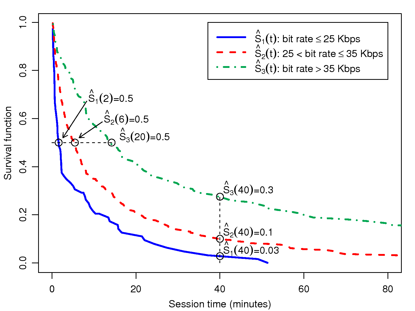
Figure 2: Survival curves for sessions with different
bit rate levels
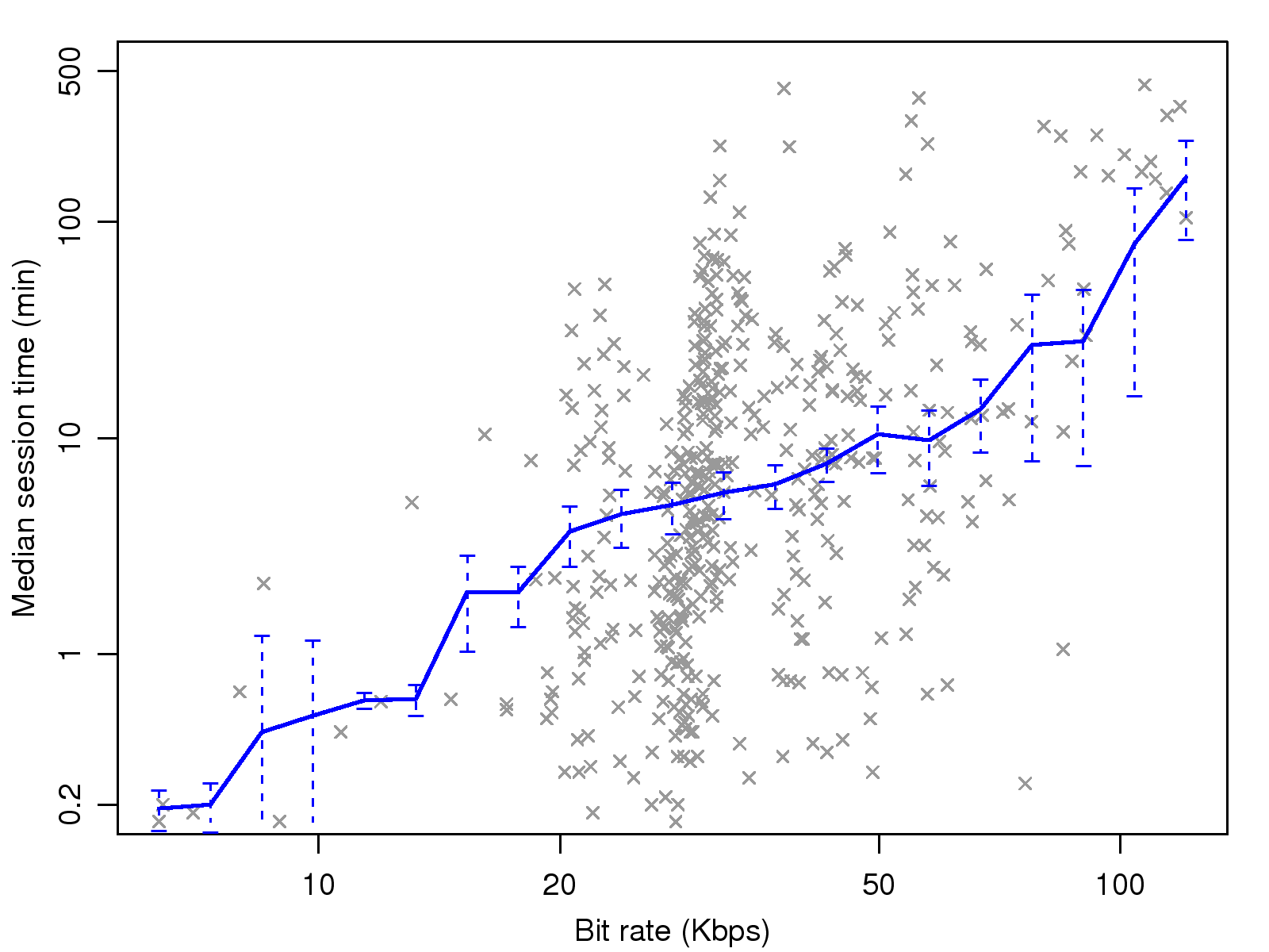
Figure 3: Correlation of bit rate with session
time
We begin with a fundamental question: "Does call duration
differ significantly with different bit rates?" To answer this
question, we use the estimated survival functions for sessions
with different bit rates. In Fig. 2, the survival
curves of three session groups, divided by 25 Kbps (15%) and
35 Kbps (60%), are plotted. The median session time of
groups 1 and 3 are 2 minutes and 20 minutes, respectively,
which gives a high ratio of 10. We can highlight this
difference in another way: while 30% of calls with bit rates
> 35 Kbps last for more than 40 minutes, only 3% of calls
hold for the same duration with low bit rates ( < 25 Kbps).
The Mantel-Haenszel test (also known as the log-rank
test) [8] is commonly used to judge whether a
number of survival functions are statistically equivalent. The
log-rank test, with the null hypothesis that all the survival
functions are equivalent, reports p=1−Prχ2,2(58) ≈ 2.7e−13, which strongly suggests that call duration varies with
different levels of bit rate. To reveal the relationship between the
bit rate and call duration in more detail, the median time and their
standard errors of sessions with increasing bit rates are plotted in
Fig. 3. The trend of median duration shows a
strong, consistent, positive, correlation with the bit rate. Before
concluding that the bit rate has a pronounced effect on call
duration, however, we remark that the same result could also be
achieved if Skype always chooses a low bit rate initially, and
increases it gradually. The hypothesis is not proven because a
significant proportion of sessions (7%) are of short duration
( < 5 minutes) and have a high bit rate ( > 40 Kbps).
4.3 Effect of Network Conditions
In addition to the source rate, network conditions are also
considered to be one of the primary factors that affect voice
quality. In order not to disturb the conversation of the Skype users,
the RTT probes (cf. Section 3.4)
were sent at 1 Hz, a frequency that is too low to capture delay
jitters due to queueing and packet loss. So we must seek some other
metric to grade the interference of the network. Given that 1) Skype
generates VoIP packets regularly, and 2) the frequency of VoIP
packets is relatively high, so the fluctuations in the data rate
observed at the receiver should reflect network delay variations to
some extent. Therefore, we use the standard deviation of the bit
rate sampled every second to represent the degree of network delay
jitters and packet loss. For brevity, we use jitter to denote the
standard deviation of the bit rate, and packet rate jitter, or
pr.jitter, to denote the standard deviation of the packet rate.
4.3.1 Effect of Round-Trip Times
We divide sessions into three equal-sized groups based on their RTTs,
and compare their lifetime patterns with the estimated survival
functions. As a result, the three groups differ significantly
(p=3.9e−6). The median duration of sessions with RTTs > 270 ms
is 4 minutes, while sessions with RTTs between 80 ms and
270 ms and sessions with RTTs < 80 ms have median duration of
5.2 and 11 minutes, respectively.
4.3.2 Effect of Jitter
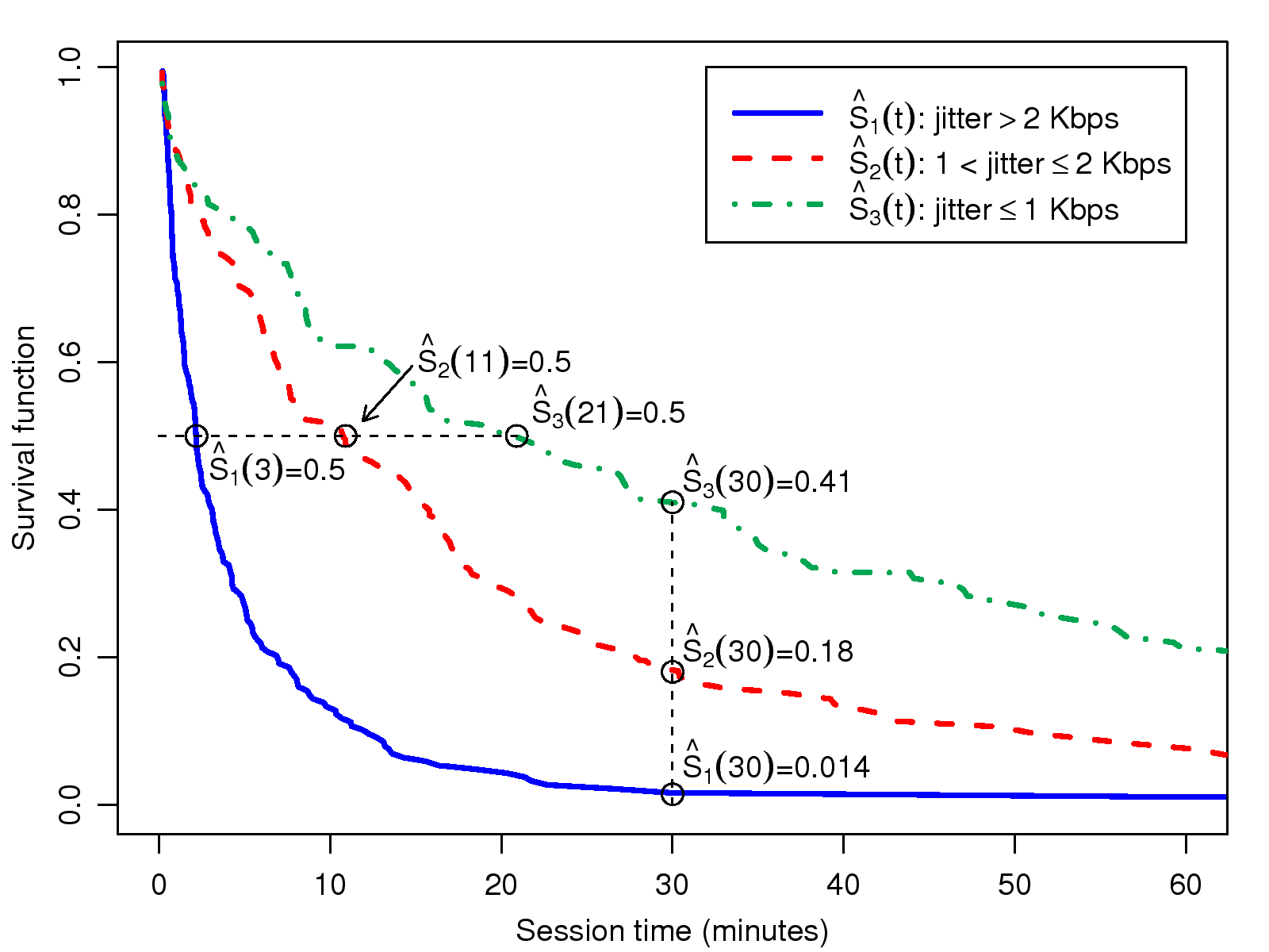
Figure 4: Survival curves for sessions with
different levels of jitter
We find that variable jitter, which captures the level of
network delay variations and packet loss, has a much higher
correlation with call duration than round-trip times. As shown in
Fig. 4, the three session groups, which are
divided by jitters of 1 Kbps and 2 Kbps, have median time of
3, 11, and 21 minutes, respectively. The p-value of the
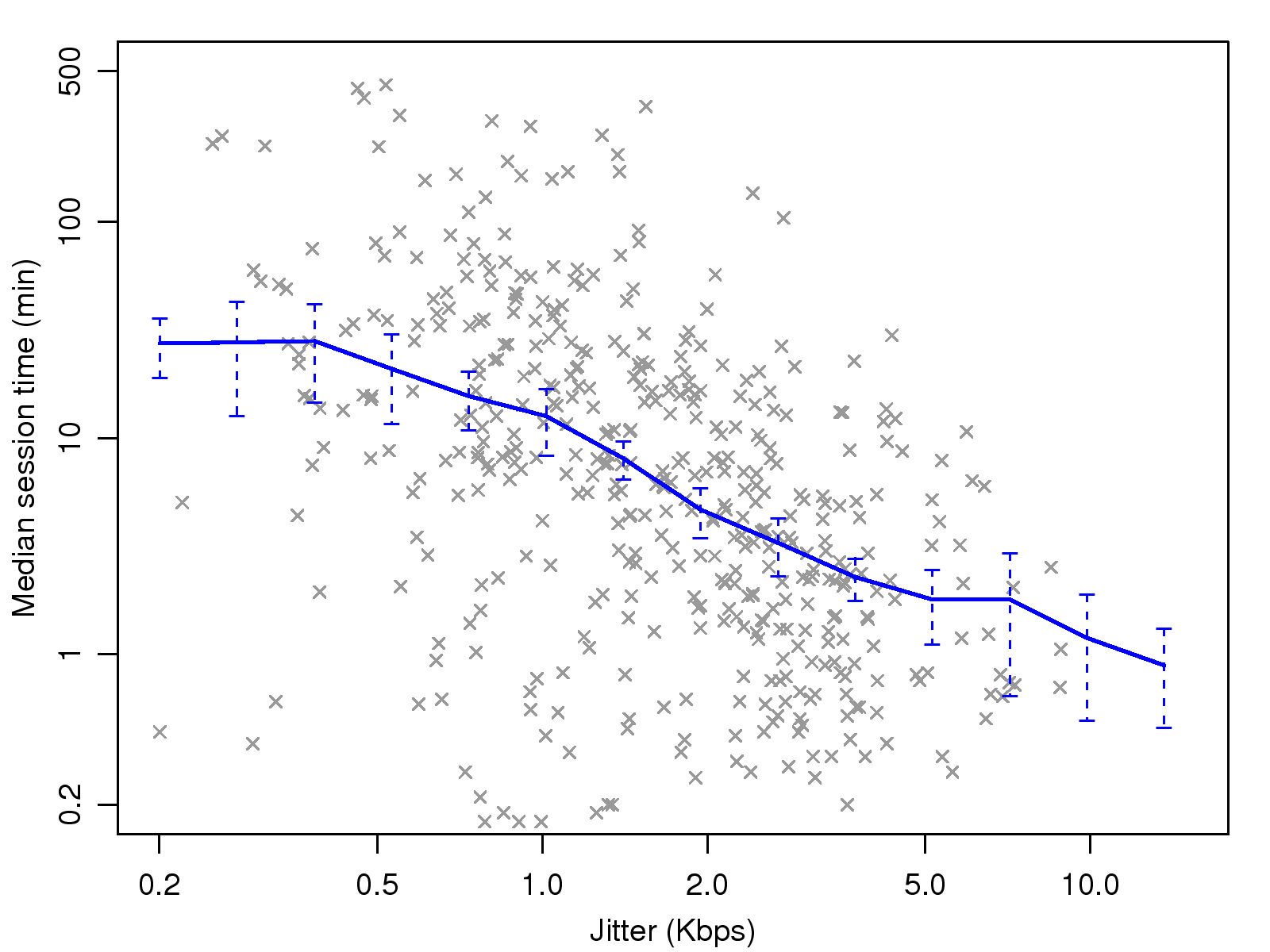
equivalence test of these groups is 1−Prχ2,2(154) ≈ 0. The correlation plot, depicted in
Fig. 5, shows a consistent and significant
downward trend in jitter versus time. Although not very
pronounced, the jitter seems to have a "threshold" effect when
it is of low magnitude. That is, a negative correlation between
jitter and session time is only apparent when the former is
higher than 0.5 pkt/sec. Such threshold effects, often seen in
factors that capture human behavior, are plausible because
listeners may not be aware of a small amount of degradation in
voice quality.
Figure 5: Correlation of jitter with session
time
4.4 Regression Modeling
We have shown that most of the QoS factors we defined, including
the source rate, RTT, and jitter, are related to call duration.
However, we note that correlation analysis does not reveal the
true impact of individual factors because of the
collinearity of factors. For example, given that the bit rate
and jitter are significantly correlated (with p ≈ 2e−6),
if both factors are related to call duration, which one is the
true source of user dissatisfaction is unclear. Users could be
particularly unhappy because of one of the factors, or be
sensitive to both of them.
To separate the impact of individual factors, we adopt regression
analysis to model call duration as the response to QoS factors.
Given that linear regression is inappropriate for modeling call
duration, we show that the Cox model provides a statistically
sound fit for the collected Skype sessions.
Following the development of the model, we propose an index to
quantify user satisfaction and then validate the index by
prediction.
4.4.1 The Cox Model
The Cox proportional hazards model [3] has long been the
most used procedure for modeling the relationship between factors
and censored outcomes. In the Cox model, we treat QoS
factors, e.g., the bit rate, as risk factors or covariates; in
other words, as variables that can cause failures. In this model,
the hazard function of each session is decided completely
by a baseline hazard function and the risk factors related to
that session. We define the risk factors of a session as a risk
vector Z. The regression equation is defined as
h(t|Z) = h0 (t)exp(βtZ)=h0(t)exp(
p ∑ k = 1
βk Zk ),
(1)
where h(t|Z) is the hazard rate at time t for a
session with risk vector Z; h0(t) is the baseline
hazard function computed during the regression process; and
β=(β1,…,βp)t is the coefficient
vector that corresponds to the impact of risk factors. Dividing
both sides of Equation 1 by h0(t) and
taking the logarithm, we obtain
log
h(t|Z)
h0 (t)
= β1 Z1 + …+ βk Zk =
p ∑ k = 1
βk Zk = β tZ,
(2)
where Zp is the pth factor of the session. The right side of
Equation 2 is a linear combination of
covariates with weights set to the respective regression
coefficients, i.e., it is transformed into a linear
regression equation. The Cox model possesses the property that,
if we look at two sessions with risk vectors Z and
Z′, the hazard ratio (ratio of their hazard rates) is
h(t|Z)
h(t|Z′)
=
h0 (t)exp[∑k = 1p βk Zk ]
h0 (t)exp[∑k = 1p βk Z′k ]
=
exp[
p ∑ k = 1
βk (Zk − Z′k )],
(3)
which is a time-independent constant, i.e., the hazard ratio of
the two sessions is independent of time. For this reason the Cox
model is often called the proportional hazards model. On
the other hand, Equation 3 imposes the
strictest conditions when applying the Cox model, because the
validity of the model relies on the assumption that the
hazard rates for any two sessions must be in proportion all
the time.
Table 3: The directions and levels of correlation between
pairs of QoS factors
br
pr
jitter
pr.jitter
pktsize
rtt
br
∗
+++
++
+++
−
pr
+++
∗
−
−−−
+
−−
jitter
++
−
∗
+++
+++
pr.jitter
−−−
+++
∗
pktsize
+++
+
+++
∗
rtt
−
−−
∗
†+/−: positive or negative correlation.
‡ Symbol #: p-value is less than 5e-2, 1e-3, 1e-4, respectively.
4.4.2 Collinearity among Factors
Although we can simply put all potential QoS factors into a
regression model, the result would be ambiguous if the predictors
were strongly interrelated [7]. Now that we
have seven factors, namely, the bit rate (br), packet rate
(pr), jitter, pr.jitter, packet size (pktsize), and
round-trip times (rtt), we explain why not all of them can be
included in the model simultaneously.
Table 3 provides the directions and levels
of interrelation between each pair of factors, where the p-value
is computed by Kendall's τ statistic as the pairs are not
necessarily derived from a bivariate normal distribution.
However, Pearson's product moment statistic yields similar
results. We find that 1) the bit rate, packet rate, and packet
size are strongly interrelated; and 2) jitter and packet rate
jitter are strongly interrelated. By comparing the regression
coefficients when correlated variables are added or deleted, we
find that the interrelation among QoS factors is very strong so
that variables in the same collinear group could interfere with
each other. To obtain an interpretable model, only one variable
in each collinear group can remain. As a result, only the bit
rate, jitter, and RTT are retained in the model, as the first two
are the most significant predictors compared with their
interrelated variables.
4.4.3 Sampling of QoS Factors
In the regression modeling, we use a scalar value for each
risk factor to capture user perceived quality. QoS factors, such
as the round-trip delay time, however, are usually not constant,
but vary during a call. To extract a representative value for
each factor in a session, which is resemble to feature vector
extraction in pattern recognition, will be a key to how well the
model can describe the observed sessions.
Intuitively, the values averaged across the whole session time would
be a good choice. However, extreme conditions may have much more
influence on user behavior than ordinary conditions. For example,
users may hang up a call earlier because of serious network lags in
a short period, but be insensitive to mild and moderate lags that
occur all the time. To derive the most representative risk vector,
we propose three measures to account for network quality, namely,
the minimum, the average, and the maximum, by two-level sampling.
That is, the original series s is first divided into sub-series of
length w, from which network conditions are sampled. This
sub-series approach confines measure of network quality within time
spans of w, thus excludes the effect of large-scale
variations. The minimum, average, and maximum measures are then
taken from sampled QoS factors which has length ⎡|s|/w⎤.
One of the three measures will be chosen depending on their ability
to describe the user perceived experience during a call.
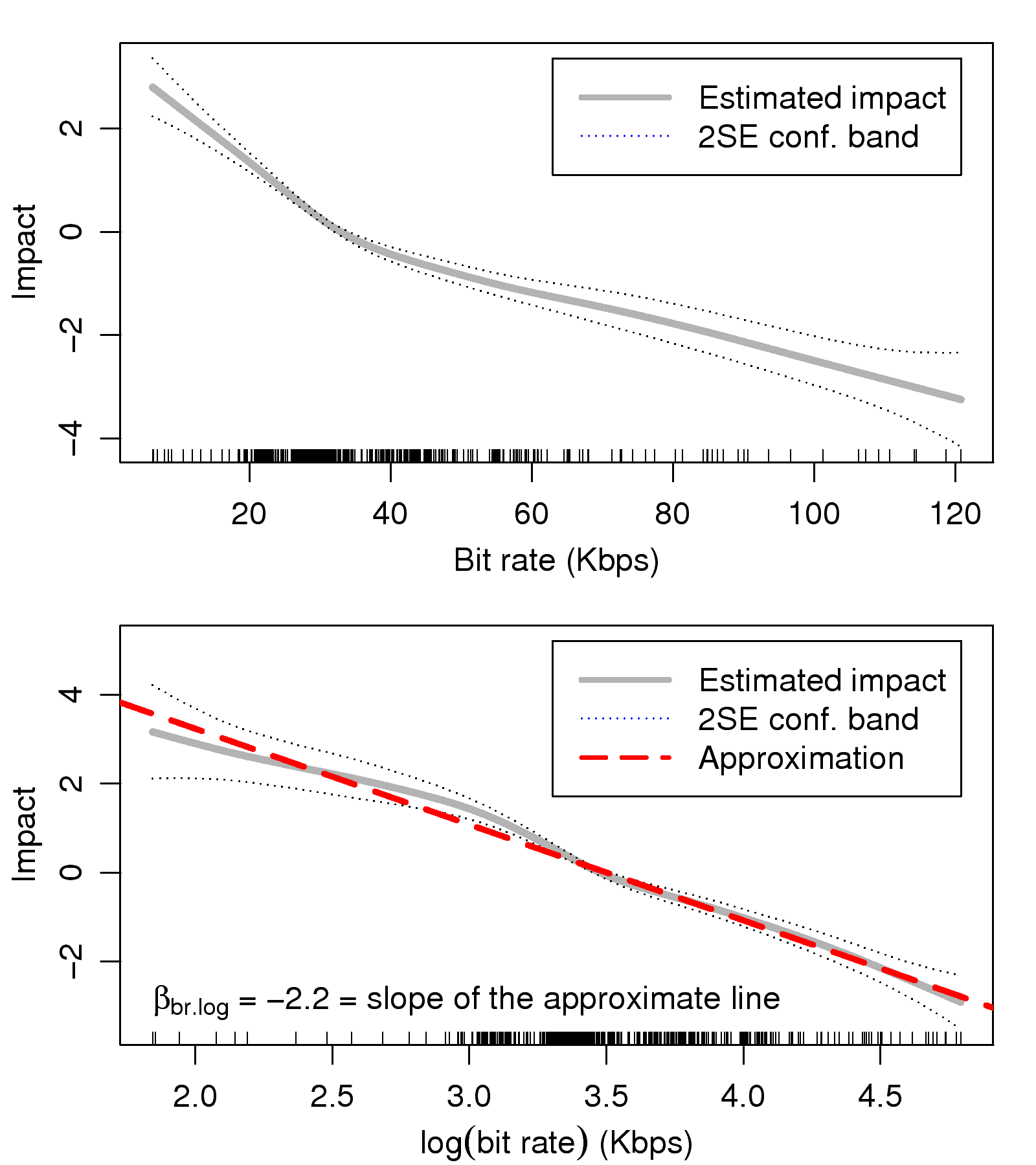
Figure 6: The functional form of the bit rate
factor
We evaluate all kinds of measures and window sizes by fitting the
extracted QoS factors into the Cox model and comparing the model's
log-likelihood, i.e., an indicator of goodness-of-fit. Finally, the
maximum bit rate and minimum jitter are chosen, both
sampled with a window of 30 seconds. The short time window implies
that users are more sensitive to short-term, rather than
long-term, behavior of network quality, as the latter may have no
influence on voice quality at all. The sampling of the bit rate,
jitter, and RTT consistently chooses the value that represents
the best quality a user experienced. This interesting finding
may be further verified by cognitive models that could determine
whether the best or the worst experience has a more dominant effect
on user behavior.
4.4.4 Model Fitting
For a continuous variable, the Cox model assumes a linear
relationship between the covariates and the hazard function,
i.e., it implies that the ratio of risks between a 20 Kbps- and a
30 Kbps-bit rate session is the same as that between a 40 Kbps-
and 50 Kbps-bit rate session. Thus, to proceed with the Cox
model, we must ensure that our predictors have a linear influence on
the hazard functions.
We investigate the impact of the covariates on the hazard
functions with the following equation:
E[si ] = exp(β t f(Z))
⌠ ⌡
∞
0
I(ti \geqslant s)h0 (s)ds,
(4)
where si is the censoring status of session i, and f(z) is
the estimated functional form of the covariate z. This corresponds
to a Poisson regression model if h0(s) is known, where the value
of h0(s) can be approximated by simply fitting a Cox model with
unadjusted covariates. We can then fit the Poisson model with
smoothing spline terms for each covariate [13]. If the
covariate has a linear impact on the hazard functions, the smoothed
terms will approximate a straight line.
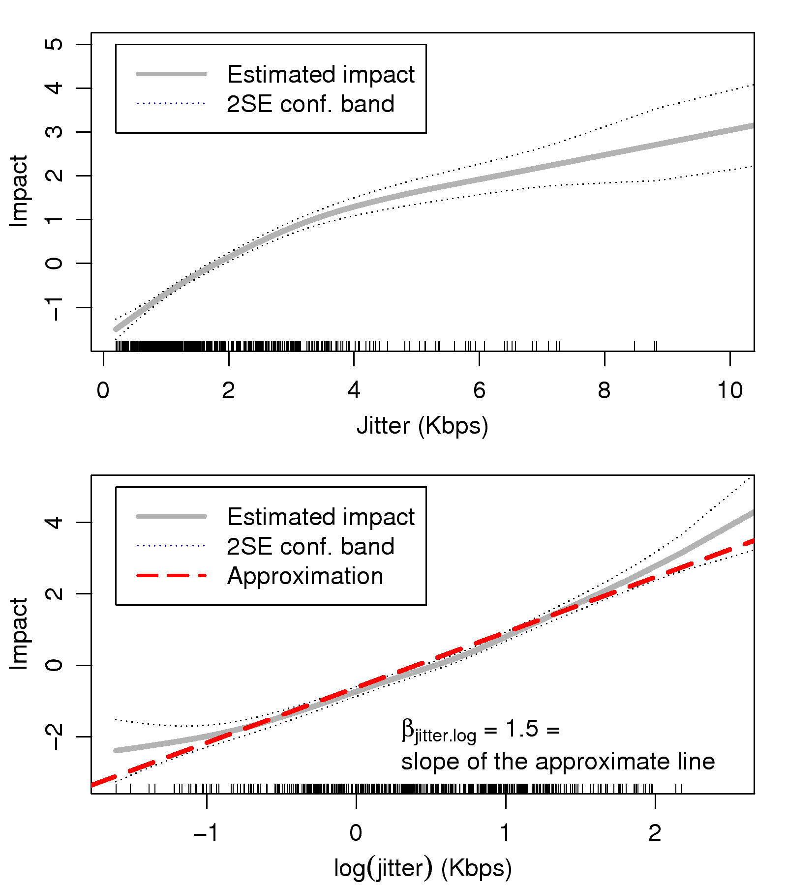
Figure 7: The functional form of the jitter
factor
In Fig. 6(a), we plot the fitted splines, as well
as their two-standard-error confidence bands, for the bit rate
factor. From the graph, we observe that the influence of the bit
rate is not proportional to its magnitude (note the change of
slope around 35 Kbps); thus, modeling this factor as linear
would not provide a good fit. A solution for non-proportional
variables is scale transformation. As shown in
Fig. 6(b), the logarithmic variable, br.log,
has a smoother and approximately proportional influence on the
failure rate. This indicates that the failure rate is
proportional to the scale of the bit rate, rather than its
magnitude. A similar situation occurs with the jitter factor,
i.e., the factor also has a non-linear impact, but its impact is
approximately linear by taking logarithms, as shown in
Fig. 7. On the other hand, the RTT factor has
an approximate linear impact so that there is no need to adjust
for it.
We employ a more generalized Cox model that allows time-dependent
coefficients [13] to check the proportional hazard
assumption by hypothesis tests. After adjustment, none of
covariates reject the linearity hypothesis at significance level
0.1, i.e., the transformed variables have an approximate linear
impact on the hazard functions. In addition, we use the Cox and
Snell residuals ri (for session i) to assess the overall
goodness-of-fit of the model [4].
We find that, except for a few sessions that have unusual call
duration,
most sessions fit the
model very well; therefore, the adequacy of the fitted model is
confirmed.
4.4.5 Model Interpretation
Table 4: Coefficients in the final model
Variable
Coef
eCoef
Std. Err.
z
P > |z|
br.log
-2.15
0.12
0.13
-16.31
0.00e+00
jitter.log
1.55
4.7
0.09
16.43
0.00e+00
rtt
0.36
1.4
0.18
2.02
4.29e-02
The regression coefficients, β, along with their standard
errors and significance values of the final model are listed in
Table 4. Contrasting them with Fig. 6
and Fig. 7 reveals that the coefficients
βbr.log and βjitter.log are simply the slopes
in the linear regression of the covariate versus the hazard
function. β can be physically interpreted by the hazard
ratios (Equation 3). For example, assuming
two Skype users call their friends at the same time with similar
bit rates and round-trip times to the receivers, but the jitters
they experience are 1 Kbps and 2 Kbps respectively, the
hazard ratio of the two calls can be computed by exp((log(2) −log(1))×βjitter.log) ≈ 2.9. That is, as long
as both users are still talking, in every instant, the
probability that user 2 will hang up is 2.9 times the
probability that user 1 will do so.
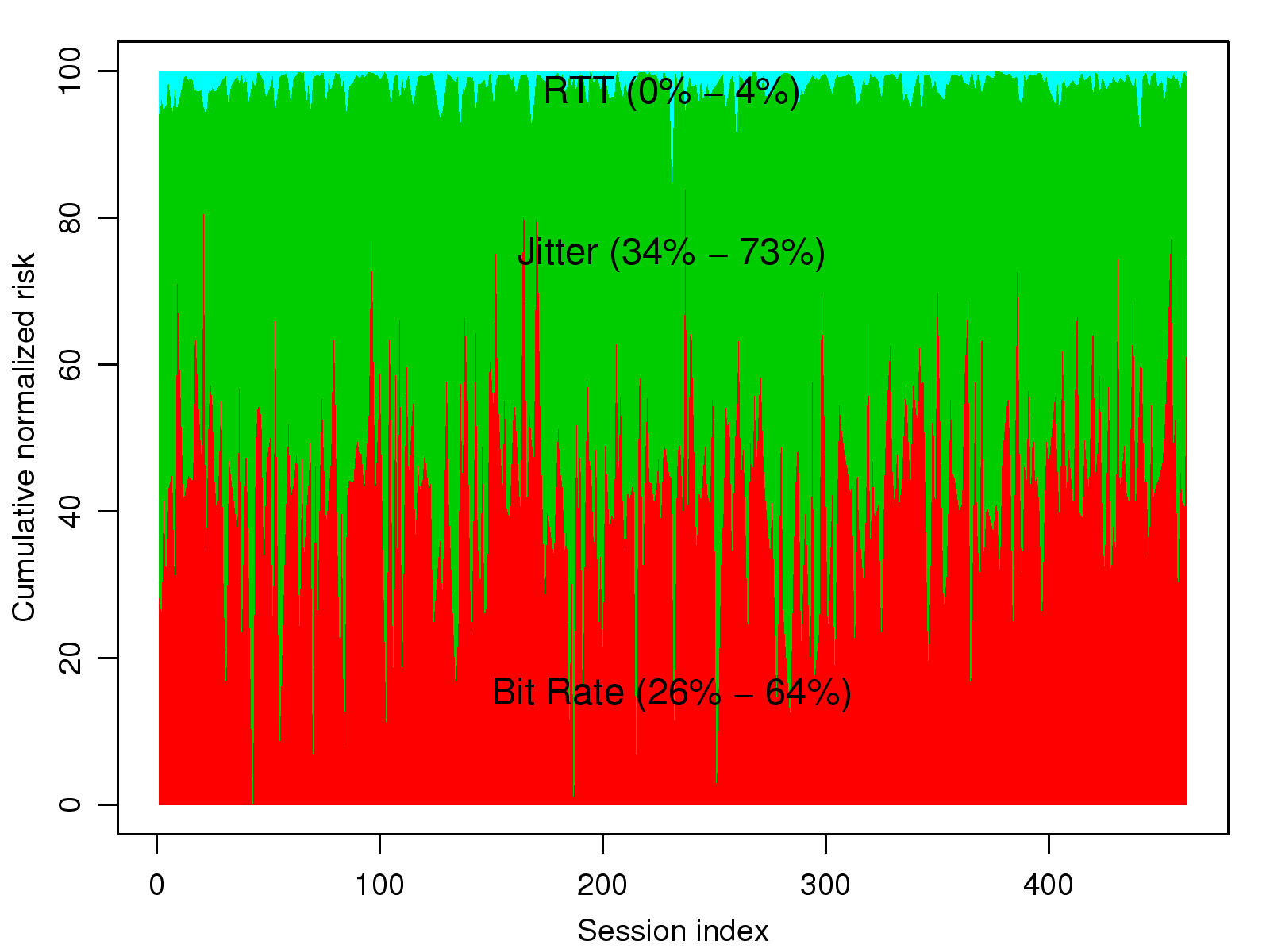
Figure 8: Relative influence of different QoS factors
for each session
The model can also be used to quantify the relative
influence of QoS factors. Knowing which factors have more impact
than others is beneficial, as it helps assign resources
appropriately to derive the maximum marginal effect in improving
users' perceived quality. We cannot simply treat β as the
relative impact of factors because they have different units. We
define the factors' relative weights as their contribution to the
risk score, i.e., βtZ. When computing the
contribution of a factor, the other factors are set to their
respective minimum values found in the trace. The relative impact
of each QoS factor, which is normalized by a total score of
100, is shown in Fig. 8. On average, the
degrees of user dissatisfaction caused by the bit rate, jitter,
and round-trip time are in the proportion of
46%:53%:1%. That is, when a user hangs up because of
poor or unfavorable voice quality, we believe that most of the
negative feeling is caused by low bit rates (46%), and high
jitter (53%), but very little is due to high round-trip times
(1%).
The result indicates that increasing the bit rate whenever
appropriate would greatly enhance user satisfaction, which is a
relatively inexpensive way to improve voice quality. We do not
know how Skype adjusts the bit rate as the algorithm is
proprietary; however, our findings show that it is possible to
improve user satisfaction by fine tuning the bit rate used.
Furthermore, the fact that higher round-trip times do not
impact on users very much could be rather a good news, as it
indicates that the use of relaying does not seriously degrade
user experience.
Also, the fact that jitters have much more impact on user perception
suggests that the choice of relay node should focus more on
network conditions, i.e., the level of congestion, rather
than rely on network latency.
4.5 User Satisfaction Index
Based on the Cox model developed, we propose the User
Satisfaction Index (USI) to evaluate Skype users' satisfaction
levels. As the risk score βtZ represents the
levels of instantaneous hang up probability, it can be seen as a
measure of user intolerance. Accordingly, we define the User
Satisfaction Index of a session as its minus risk score:
USI
=
−βtZ
=
2.15×log(bitrate)− 1.55 ×log(jitter)
− 0.36 ×RTT,
where the bit rate, jitter, and RTTs are sampled using a
two-level sampling approach as described in
Section 4.4.3.
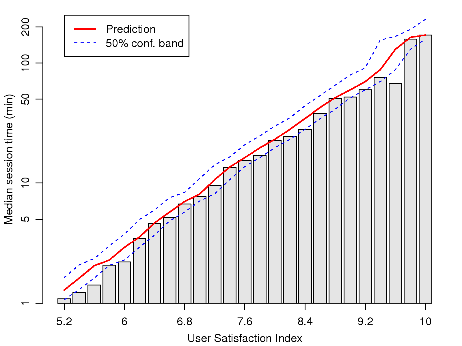
We verify the proposed index by prediction. We first group
sessions by their USI, and plot the actual median duration,
predicted duration, and 50% confidence bands of the latter for
each group, as shown in Fig. 9. The prediction
is based on the median USI for each group. Note that the y-axis
is logarithmic to make the short duration groups clearer. From
the graph, we observe that the logarithmic duration is
approximately proportional to USI, where a higher USI corresponds
to longer call duration with a consistently increasing trend.
Also, the predicted duration is rather close to the actual median
time, and for most groups the actual median time is within the
50% predicted confidence band.
Figure 9: Predicted vs. actual median duration of
session groups sorted by their User Satisfaction
Indexes.
Compared with other objective measures of sound
quality [11,9], which often require access to
voice signals at both ends, USI is particularly useful because
its parameters are readily accessible; it only requires the first
and second moments of the packet counting process, and the
round-trip times. The former can be obtained by simply counting
the number and bytes of arrived packets, while the latter are
usually available in peer-to-peer applications for overlay
network construction and path selection. Furthermore, as we have
developed the USI based on passive measurement, rather than
subjective surveys [11], it can also capture
subconscious reactions of participants, which may not be
accessible through surveys.
5 Analysis of User Interaction
In this section, we validate the proposed User Satisfaction Index by
an independent set of metrics that quantify the interactivity
and smoothness of a conversation. A smooth dialogue usually
comprises highly interactive and tight talk bursts. On the other
hand, if sound quality is not good, or worse, the sound is
intermittent rather than continuous, the level of interactivity will
be lower because time is wasted waiting for a response, asking for
for something to be repeated, slowing the pace, repeating sentences,
and thinking. We believe that the degree of satisfaction with a call
can be, at least partly, inferred from the conversation pattern.
The difficultly is that, most VoIP applications, including Skype,
do not support silence suppression; that is, lowering the
packet sending rate while the user is not talking.
This design is deliberate to maintain UDP port bindings at the NAT
and ensure that the background sound can be heard all the time.
Thus, we cannot tell whether a user is speaking or silent by simply
observing the packet rate. Furthermore, to preserve privacy, Skype
encrypts every voice packet with 256-bit AES (Advanced Encryption
Standard) and uses 1024 bit RSA to negotiate symmetric AES
keys [2]. Therefore, parties other than
call participants cannot know the content of a conversation, even if
the content of voice packets have been revealed.
Given that user activity during a conversation is not directly
available, we propose an algorithm that infers conversation patterns
from packet header traces. In the following, we first describe and
validate the proposed algorithm. We then use the voice interactivity
that capture the level of user satisfaction within a conversation to
validate the User Satisfaction Index. The results show that the USI,
which is based on call duration, and the voice interactivity
measures, which are extracted from user conversation patterns, strongly
support each other.
5.1 Inferring Conversation Patterns
Through some experiments, we found that both the packet size and bit
rate could indicate user activity, i.e., whether a user is talking
or silent. The packet size is more reliable than the bit rate, since
the latter also takes account of the packet rate, which is
independent of user speech. Therefore, we rely on the packet size
process to infer conversation patterns. However, deciding a packet
size threshold for user speech is not trivial because the packet
sizes are highly variable. In addition to voice volume, the packet
size is decided by other factors, such as the encoding rate, CPU
load, and network path characteristics, all of which could vary over
time. Thus, we cannot determine the presence of speech bursts by
simple static thresholding.
We now introduce a dynamic thresholding algorithm that is based on
wavelet denoising [6]. We use wavelet denoising
because packet sizes are highly variable, a factor affected by
transient sounds and the status of the encoder and the network.
Therefore, we need a mechanism to remove high-frequency
variabilities in order to obtain a more stable description of
speech. However, simple low-pass filters do not perform well because
a speech burst could be very short, such as "Ah," "Uh," and
"Ya," and short bursts are easily diminished by averaging.
Preserving such short responses is especially important in our
analysis as they indicate interaction and missing them leads to
underestimation of interactivity. On the other hand, wavelet
denoising can localize higher frequency components in the time
domain better; therefore, it is more suitable for our scenario,
since it preserves the correct interpretation of sub-second speech
activity.
5.1.1 Proposed Algorithm
Our method works as follows. The input is a packet size process,
called the original process, which is averaged every 0.1 second.
For most calls, packets are generated at a frequency of
approximately 33 Hz, equivalent to about three packets per sample.
We then apply the wavelet transform using the index 6 wavelet in
the Daubechies family [5], which is widely used
because it relatively easy to implement. The denoising operation is
performed by soft thresholding [6] with threshold
T=σ√{2logN}, where σ is the standard deviation
of the detail signal and N denotes the number of samples. To
preserve low-frequency fluctuations, which represent users' speech
activity, the denoising operation only applies to time scales
smaller than 1 second.
In addition to fluctuations caused by users' speech activity, the
denoised process contains variations due to low-frequency network
and application dynamics. Therefore, we use a dynamic
thresholding method to determine the presence of speech bursts.
We first find all the local extremes, which are the local maxima
or minima within a window larger than 5 samples. If the maximum
difference between a local extreme and other samples within the
same window is greater than 15 bytes, we call it a "peak" if
it is a local maxima, and a "trough" if it is a local minima.
Once the peaks and troughs have been identified, we compute the
activity threshold as follows.
We denote each peak or trough i occurring at time ti with an
average packet size si as (ti, si). For each pair of adjacent
troughs (tl, sl) and (tr, sr), if there are one or more
peaks P in-between them, and the peak p ∈ P
has the largest packet size, we draw an imaginary line from (tl,(sl+sp)/2) to (tr, (sr+sp)/2) as the binary threshold of
user activity. Finally we determine the state of each sample as ON
or OFF, i.e., whether a speech burst is present, by checking whether
the averaged packet size is higher than any of the imaginary
thresholds.
Figure 10: Network setup for obtaining realistic packet
size processes generated by Skype
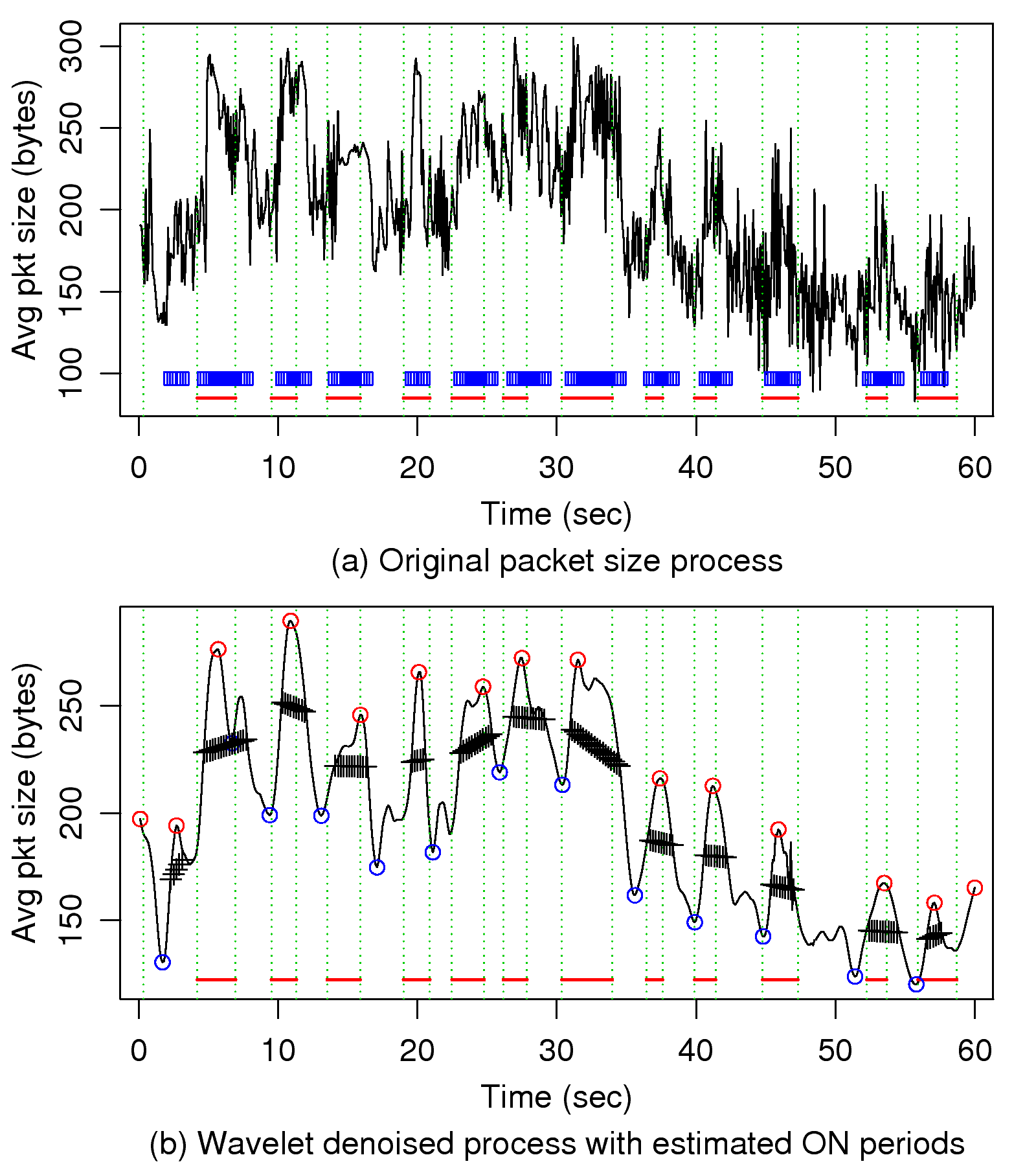
5.1.2 Validation by Synthesized Wave
Figure 11: Verifying the speech detection algorithm
with synthesized ON/OFF sine waves
We first validate the proposed algorithm with synthesized wave
files. The waves are sampled at 22.5 KHz frequency with 8 bit
levels. Each wave file lasts for 60 seconds and comprises
alternate ON/OFF periods with exponential lengths of mean 2
seconds. The ON periods are composed of sine waves with the
frequency uniformly distributed in the range of 500 to 2000
Hz, where the OFF periods do not contain sound.
To obtain realistic packet size processes that are contaminated by
network impairment, i.e., queueing delays and packet loss, we
conducted a series of experiments that involved three Skype nodes.
As shown in Fig. 10, we establish a VoIP session
between two local Skype hosts and force them to connect via a relay
node by blocking their intercommunication with a firewall. The
selection of relay node is out of our control because it is chosen
by Skype. The relay node used is far from our Skype hosts with
transoceanic links in-between and an average RTT of approximately
350 ms, which is much longer than the average 256 ms. Also, the
jitter our Skype calls experienced is 5.1 Kbps,
which is approximately the 95 percentile in the collected
sessions. In the experiment, we play synthesized wave files to the
input of Skype on the sender, and take the packet size processes on
the receiver. Because the network characteristics in our experiment
are much worse than the average case in collected sessions, we
believe the result of the speech detection here would be close to
the worst case, as the measured packet size processes contain so
much variation and unpredictability.
To demonstrate, the result of a test run is shown in
Fig. 11. The upper graph depicts the original
packet size process with the red line indicating true ON periods
and blue checks indicating estimated ON periods. The lower graph
plots the wavelet denoised version of the original process, with
red and blue circles marking the location of peaks and troughs,
respectively. The oblique lines formed by black crosses are
binary thresholds used to determine speech activity. As shown by
the figure, wavelet denoising does a good job in removing
high-frequency variations that could mislead threshold decisions,
but retains variations due to user speech. Note that long-term
variation is present because the average packet size used in the
second half of the run is significantly smaller than that in the
first half. This illustrates the need for dynamic thresholding,
as the packet size could be affected by many factors other than
user speech.
Totally 10 test cases are generated, each of which is run 3
times. Since we have the original waves, the correctness of the
speech detection algorithm can be verified. Each test is divided
into 0.1-second periods, the same as the sampling interval, for
correctness checks. Two metrics are defined to judge the accuracy
of estimation: 1) Correctness: the ratio of matched periods,
i.e., the periods whose states, either ON or OFF, are correctly
estimated; and 2) the number of ON periods. As encoding,
packetization, and transmission of voice data necessarily
introduce some delay, the correctness is computed with time
offsets ranging from minus one to plus one second, and the
maximum ratio of the matched periods is used. The experiment
results show that the correctness ranges from 0.73-0.92 with
a mean of 0.8 and standard deviation of 0.05. The estimated
number of ON periods is always close to the the actual number of
ON periods; the difference is generally less than 20% of the
latter. Although not perfectly exact, the validation experiment
shows that the proposed algorithm estimates ON/OFF periods with
good accuracy, even if the packet size processes have been
contaminated by network dynamics.
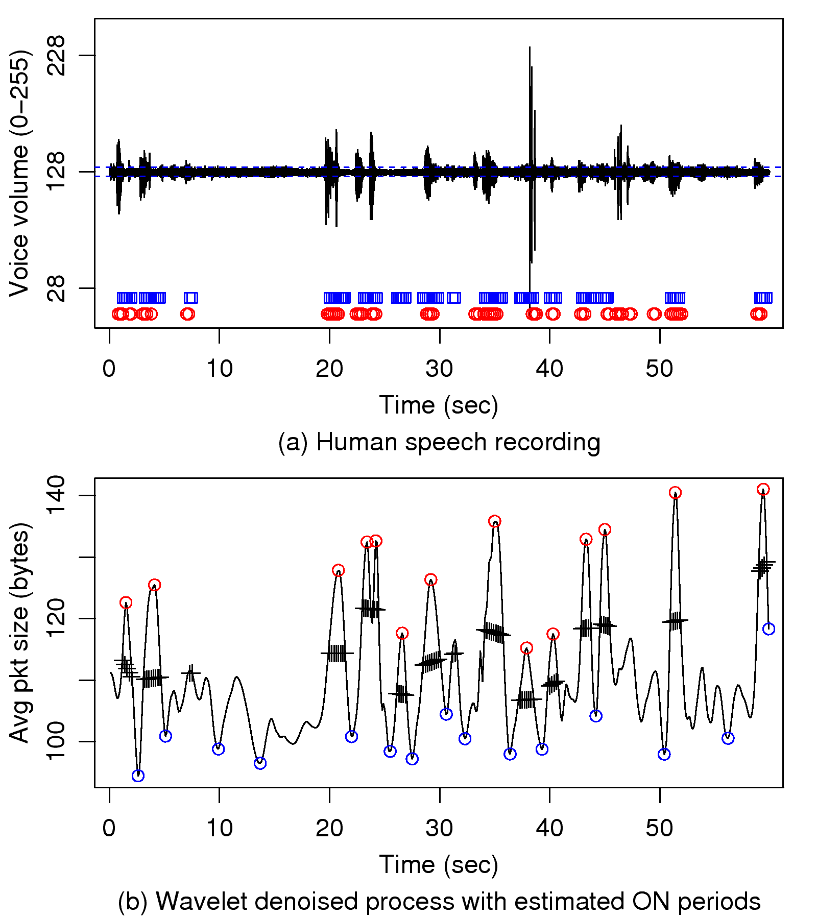
5.1.3 Validation by Speech Recording
Figure 12: Verifying the speech detection
algorithm with human speech recordings
Since synthesized ON/OFF sine waves may be very different from
human speech, we further experiment with human speech recordings.
We repeat the preceding experiment by replacing synthesized wave
files with human speech recorded via microphone during phone calls.
Given that the sampled voice levels range from 0 to 255, with
the center at 128, we use an offset of +/−4 to indicate
whether a specific volume corresponds to audible sounds. Among a
total of 9 runs for three test cases, the correctness
ranges from 0.71 to 0.85. The number of ON periods differs
from true values by less than 32%. The accuracy of detection
is slightly worse than the experiment with synthesized waves, but
still correctly captures most speech activity.
Fig. 12 illustrates the result of one test,
which shows that the algorithm detects speech bursts reasonably
well, except for the short spikes around 47 seconds.
5.2 User Satisfaction Analysis
To determine the degree of user satisfaction from conversation
patterns, we propose the following three voice interactivity
measures to capture the interactivity and smoothness of a given
conversation:
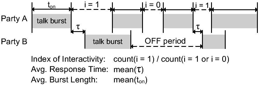
Responsiveness: A smooth conversation usually
involves alternate statements and responses. We measure the
interactivity by the degree of "alternation," that is, the
proportion of OFF periods that coincide with ON periods of the
other side, as depicted in Fig. 13. Since the
level of interactivity is computed separately for each direction,
the minimum of both is used because it represents the worse
satisfaction level.
Response Delay: Short response delay, i.e., one side
responds immediately after the other side stops talking, usually
indicates the sound quality is good enough for the parties to
understand each other. Thus, if one side starts talking when the
other side is silent, we consider it as a "response" to the
previous burst from the other side, and take the time difference
between the two adjacent bursts as the response delay, as depicted
in Fig. 13. In this way, all the response delays
in the same direction can be averaged, and the larger of the
average response delays in both directions is used, since longer
response delay indicates poorer conversation quality.
Talk Burst Length: This definition may not be
intuitive at first glance.
We believe that people usually adapt to low voice quality by
slowing their talking speed, as this should help the other
side understand. Furthermore, if people need to repeat an idea
due to poor sound quality, they tend to explain the idea in
another way, which is simpler, but possibly longer. Both of the
above behavior patterns lead to longer speech bursts. We capture
such behavior by the larger of the average burst lengths in both
directions, as longer bursts indicate poorer quality. In order
not to be biased by long bursts, which are due to lengthy speech
or error-estimation in the speech detection, only bursts shorter
than 10 seconds are considered.
Figure 13: Proposed measures for voice interactivity, which indicate user
satisfaction from conversation patterns
Fig. 13 illustrates the voice interactivity
measures proposed. Because our speech detection algorithm estimates
talk bursts in units of 0.1 second, a short pause between words or
sentences, either intentional or unintentional, could split one
burst into two. To ensure that the estimated user activity resembles
true human behavior, we treat successive bursts as a single burst if
the intervals between them are shorter than 1 second in the
computation of the interactivity measures. We summarize some
informative statistics and voice interactivity measures of the
collected
sessions in Table 5.
Table 5: Summary statistics for conversation patterns in the collected
sessions
Statistic
Mean
Std. Dev.
ON Time
70.8%
9.5%
# ON Rate (one end)
3.9 pr/min
1.2 pr/min
# ON Rate (both ends)
6.4 pr/min
1.9 pr/min
Responsiveness
0.90
0.11
Avg. Response Time
1.4 sec
0.5 sec
Avg. Burst Length
2.9 sec
0.7 sec
Now that we have 1) the User Satisfaction Index
(Section 4.5), which is based on the call duration
compared to the network QoS model, and 2) the interactivity measures,
which are inferred from the speech activity in a call.
Since these two indexes are obtained independently in
completely different ways, and the speech detection algorithm does
not depend on any parameter related to call duration, we use them to
cross validate their representativeness of each other. In the
following, we check the correlation between the USI and the voice
interactivity measures with both graphical plots and correlation
coefficients.
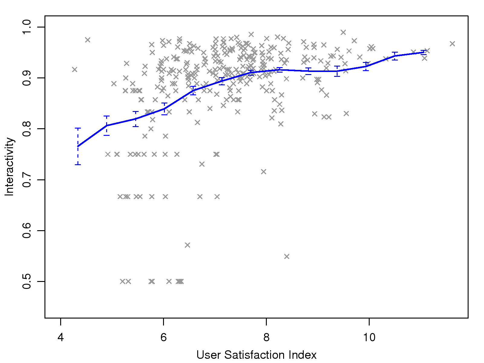
(a) Responsiveness vs. USI
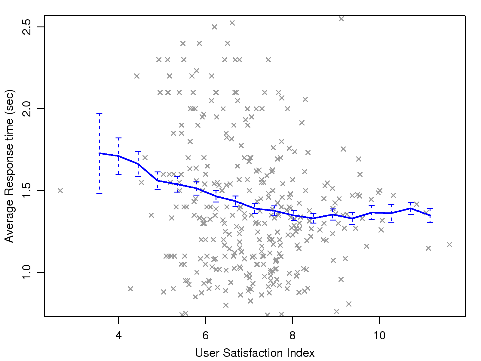
(b) Average response delay vs. USI
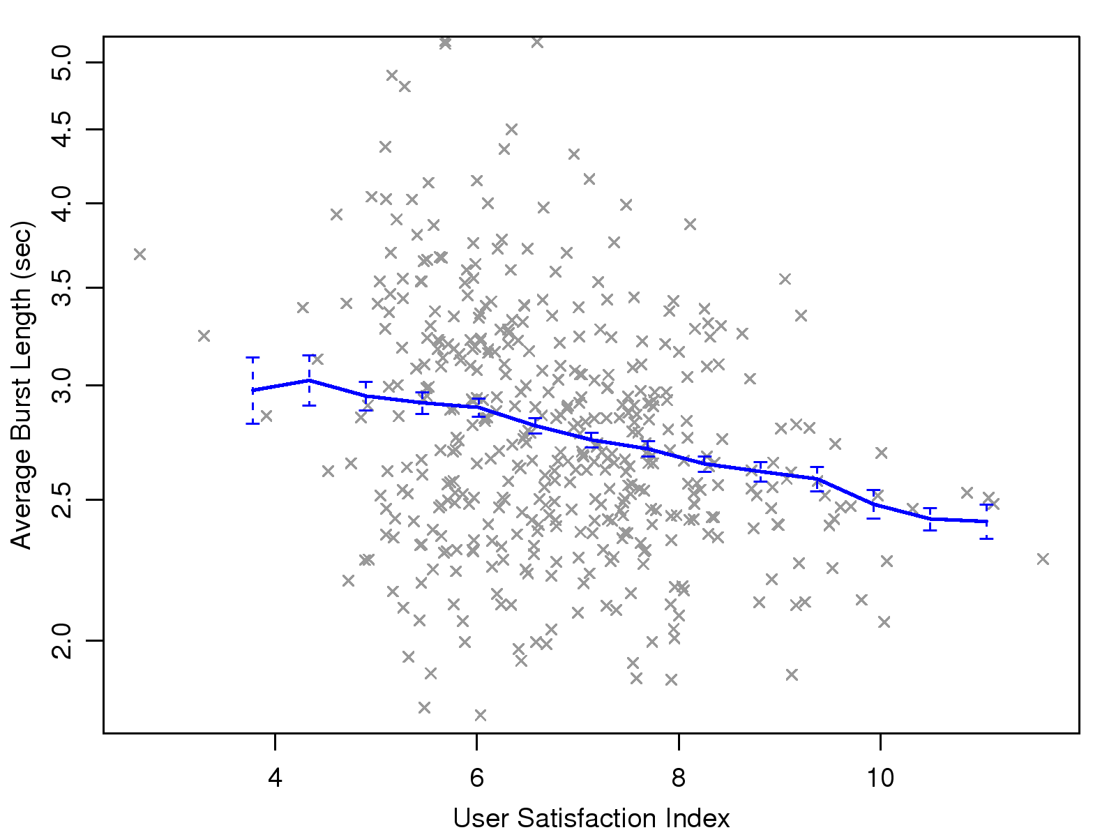
(c) Average talk burst length vs.
USI
Figure 14: The correlation between voice interactivity measures and USI.
First, we note that short sessions, i.e., shorter than 1 minute,
tend to have very high indexes of responsiveness, possibly because
both parties attempt to speak regardless of the sound quality during
such a short conversation. Accordingly, we ignore extreme cases
whose responsiveness level equals one. The scatter plot of the USI
versus responsiveness is shown in Fig. 14(a). In
the graph, the proportion of low-responsiveness sessions decreases
as the USI increases, which supports our intuition that a higher USI
indicates higher responsiveness.
Fig. 14(b) shows that response delays are also
strongly related to the USI, as longer response delay corresponds
to lower USI. The plot shows a threshold effect in that the
average response delay does not differ significantly for USIs
higher than 8. This is plausible, as response delay certainly
does not decrease unboundedly, even if the voice quality is
perfect.
Fig. 14(c) shows that the average talk burst length
consistently increases as the USI drops. As explained earlier, we
consider that this behavior is due to the slow-paced
conversations and longer explanations caused by poor sound
quality.
We also performed statistical tests to confirm the association
between the USI and the voice interactivity measures. Three measures,
Pearson's product moment correlation coefficient, Kendall's
τ, and Spearman's ρ, were computed, as shown in
Table 6. All correlation tests reject the null
hypothesis that an association does not exist at the 0.01
level. Furthermore, the three tests support each other with
coefficients of the same sign and approximate magnitude.
Table 6: Correlation tests of the USI and voice interactivity measures
Pearson
Kendall
Spearman
Responsiveness
0.36**
0.27**
0.39**
Avg. Resp. Delay
−0.20**
−0.10**
−0.16**
Avg. Burst Length
−0.27**
−0.18**
−0.26**
† ** The p-value of the correlation test is < 0.01.
6 Conclusion
Understanding user satisfaction is essential for the development
of QoS-sensitive applications. The proposed USI model captures
the level of satisfaction without the overheads of the
traditional approaches, i.e., requiring access to speech signals.
It also captures factors other than signal degradation, such as
talk echo, conversational delay, and subconscious reactions.
Results of the validation tests using a set of independent
measures derived from user interactivities show a strong
correlation between the call durations and user interactivities.
This suggests that the USI based on call duration is
significantly representative of Skype user satisfaction.
The best feature of the USI is that its parameters are easily
accessible and computable online. Therefore, in addition to
evaluating the performance of QoS-sensitive applications, the USI
can be implemented as part of applications to allow adaptation
for optimal user satisfaction in real time.
Acknowledgments
The authors would like to acknowledge anonymous referees for their
constructive criticisms.
References
[1]
S. A. Baset and H. Schulzrinne.
An analysis of the Skype peer-to-peer internet telephony protocol.
In Proceedings of IEEE INFOCOM'06, Barcelona, Spain, Apr. 2006.
[2]
T. Berson.
Skype security evaluation.
ALR-2005-031, Anagram Laboratorie, 2005.
[3]
D. R. Cox and D. Oakes.
Analysis of Survival Data.
Chapman & Hall/CRC, June 1984.
[4]
D. R. Cox and E. J. Snell.
A general definition of residuals (with discussion).
Journal of the Royal Statistical Society, B 30:248-275, 1968.
[5]
I. Daubechies.
The wavelet transform, time-frequency localization and signal
analysis.
IEEE Transactions on Information Theory, 36(5):961-1005, Sept.
1990.
[6]
D. L. Donoho.
De-noising by soft-thresholding.
IEEE Transactions on Information Theory, 41(3):613-627, May
1995.
[7]
F. E. Harrell.
Regression Modeling Strategies, with Applications to Linear
Models, Survival Analysis and Logistic Regression.
Springer, 2001.
[8]
D. P. Harrington and T. R. Fleming.
A class of rank test procedures for censored survival data.
Biometrika, 69:553-566, 1982.
[9]
ITU-T Recommendation P.862.
Perceptual evaluation of speech quality (PESQ), an objective method
for end-to-end speech quality assessment of narrow-band telephone networks
and speech codecs, Feb 2001.
[10]
K. Lam, O. Au, C. Chan, K. Hui, and S. Lau.
Objective speech quality measure for cellular phone.
In Proceedings of IEEE International Conference on Acoustics,
Speech, and Signal Processing, volume 1, pages 487-490, 1996.
[11]
A. Rix, J. Beerends, M. Hollier, and A. Hekstra.
Perceptual evaluation of speech quality (PESQ) - a new method for
speech quality assessment of telephone networks and codecs.
In Proceedings of IEEE International Conference on Acoustics,
Speech, and Signal Processing, volume 2, pages 73-76, 2001.
[12]
K. Suh, D. R. Figueiredo, J. Kurose, and D. Towsley.
Characterizing and detecting relayed traffic: A case study using
Skype.
In Proceedings of IEEE INFOCOM'06, Barcelona, Spain, Apr. 2006.
[13]
T. M. Therneau and P. M. Grambsch.
Modeling Survival Data: Extending the Cox Model.
Springer, 1st edition, August 2001.
 (a) Responsiveness vs. USI
 (b) Average response delay vs. USI
 (c) Average talk burst length vs.
USI
(c) Average talk burst length vs.
USI